
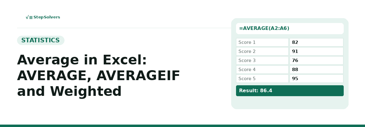
To calculate an average in Excel, type =AVERAGE(A2:A6) into an empty cell, replace the range with your own data, and press Enter. Excel adds up the numbers and divides by how many there are. For a condition, such as the average of one region only, use AVERAGEIF. For a weighted average, use SUMPRODUCT divided by SUM.
The AVERAGE Function Step by Step
- Enter your numbers in one column, one value per cell (for example, cells A2 through A6).
- Click an empty cell where you want the result.
- Type
=AVERAGE(A2:A6), adjusting the range to match your data. - Press Enter. Excel returns the mean straight away.
You can also select the numbers and look at the status bar at the bottom of the Excel window. It shows the average, the count and the sum of the selected cells without typing anything. If you do not see Average there, right-click the status bar and tick it.
Worked Example
Take five test scores: 82, 91, 76, 88 and 95, entered in cells A2 to A6.
| Cell | Value |
|---|---|
| A2 | 82 |
| A3 | 91 |
| A4 | 76 |
| A5 | 88 |
| A6 | 95 |
Behind the scenes, Excel adds the values (82 + 91 + 76 + 88 + 95 = 432) and divides by the count of numbers (5).
Which Excel Average Function Should You Use?
| Function | What it does | Example |
|---|---|---|
| AVERAGE | Mean of the numbers in a range. Ignores blanks and text, counts zeros. | =AVERAGE(B2:B6) |
| AVERAGEIF | Mean of the cells that meet one condition. | =AVERAGEIF(A2:A6,"East",B2:B6) |
| AVERAGEIFS | Mean of the cells that meet several conditions. | =AVERAGEIFS(B2:B6,A2:A6,"East",B2:B6,">100") |
| AVERAGEA | Like AVERAGE, but counts text as 0 and TRUE as 1. | =AVERAGEA(B2:B6) |
| SUMPRODUCT / SUM | Weighted average. | =SUMPRODUCT(B2:B4,C2:C4)/SUM(C2:C4) |
| MEDIAN and MODE.SNGL | The middle value and the most frequent value. | =MEDIAN(B2:B6) |
Average with a Condition: AVERAGEIF
Suppose column A holds a region and column B holds sales: East 120, West 90, East 150, West 110, East 135 (rows 2 to 6). To average only the East sales:
The three East values are 120, 150 and 135, which add up to 405, so the average is 405 ÷ 3 = 135. The West average is (90 + 110) ÷ 2 = 100. Note the argument order: AVERAGEIF takes the criteria range first and the range to average last, while AVERAGEIFS takes the range to average first.
You can also test the numbers themselves. =AVERAGEIF(B2:B6,">100") averages only the sales above 100 (120, 150, 110 and 135), giving 515 ÷ 4 = 128.75. To ignore zeros in a list, use =AVERAGEIF(B2:B6,"<>0").
Weighted Average in Excel
When some values count more than others, such as course grades with different credit weights, a plain average is wrong. Excel has no weighted average function, so divide the weighted total by the total weight:
Here column B holds the values and column C holds the weights. SUMPRODUCT multiplies each value by its weight and adds the results, and SUM adds the weights.
How to Average Averages Correctly
A very common mistake is averaging a list of averages. It only works when every group has the same number of items. Say Class A has 10 students with an average of 70, and Class B has 30 students with an average of 90.
| Class | Average (B) | Students (C) |
|---|---|---|
| A | 70 | 10 |
| B | 90 | 30 |
=AVERAGE(B2:B3)gives 80, which is wrong because it treats the classes as equal in size.=SUMPRODUCT(B2:B3,C2:C3)/SUM(C2:C3)gives (700 + 2,700) ÷ 40 = 85, which is the true average of all 40 students.
Common Mistakes and Errors
- Numbers stored as text.
AVERAGEskips them, so the result looks too high or turns into#DIV/0!when no real numbers are found. Look for a green corner triangle, then convert the cells to numbers. - Zeros you did not mean to count. A zero is a real number to Excel and lowers the mean. If a zero means "no data", exclude it with
AVERAGEIF(range,"<>0"). - Averaging hidden or filtered rows.
AVERAGEincludes manually hidden rows. Use=SUBTOTAL(101,range)to leave them out. - Picking the mean when the data is skewed. A few very large values can drag the average up. Compare it with
=MEDIAN(range)before reporting it.
If you want the mean, median, mode and every step of the working without building a sheet, try the Average Calculator. To go from the average to how spread out the data is, see how to calculate standard deviation in Excel and what variance is.
Frequently Asked Questions
- How do I calculate the average in Excel?
- Type =AVERAGE(A2:A6) in an empty cell, replacing A2:A6 with your own range, and press Enter. Excel adds up the numbers in the range and divides by how many numbers there are. For the scores 82, 91, 76, 88 and 95, the result is 86.4.
- How do I calculate an average of averages in Excel?
- Do not simply average the averages, because that treats every group as the same size. Multiply each group's average by its count, add the results, and divide by the total count: =SUMPRODUCT(averages, counts)/SUM(counts). Two classes averaging 70 (10 students) and 90 (30 students) give 85, not 80.
- Does Excel's AVERAGE function ignore blank cells and zeros?
- AVERAGE ignores blank cells and text, but it counts zeros as real numbers, so a zero pulls the average down. To leave zeros out, use =AVERAGEIF(range,"<>0").
- What is the difference between AVERAGE and AVERAGEA?
- AVERAGE ignores text and logical values in a range. AVERAGEA counts text as 0, TRUE as 1 and FALSE as 0, so it usually returns a lower number when the range contains text. Use AVERAGE for ordinary numeric data.
- How do I calculate a weighted average in Excel?
- Use =SUMPRODUCT(values, weights)/SUM(weights). Excel has no built-in weighted average function, but this formula multiplies each value by its weight, adds the products, and divides by the total weight.
- Why does my AVERAGE formula show #DIV/0!?
- The range has no numbers in it. This usually happens when the numbers are stored as text (often shown with a green corner triangle) or the range is empty. Convert the text to numbers, or use =IFERROR(AVERAGE(range),"") to show a blank instead of the error.